Math Refresher: Linear Algebra

Quantum states live in a vector space, and observables act on them as matrices. This page defines the pieces: vectors, matrix multiplication, the adjoint, eigenvalues, and the bra-ket notation that carries them.

1. Vectors

A vector is an ordered list of numbers. A column vector with two entries is

$$\mathbf{v}=\left(\begin{array}{c}{v}_1\\ v_2\end{array}\right).$$

The entries are its components in some basis. Adding two vectors adds component by component, and multiplying by a number scales every component. These two operations are what "vector space" means, so a quantum state — a vector in Hilbert space — can be added to another and scaled, exactly like an arrow.

The entries are complex numbers in general, because quantum amplitudes carry a phase. Real vectors are the special case in which every imaginary part is zero; throughout these pages, components such as $v_1$ and $v_2$ are complex unless stated otherwise. That is what makes the conjugation in §3 and §5 necessary.

Vectors are independent if none of them is a combination of the others. A basis is an independent set that spans the space, meaning every vector is a unique combination of the basis vectors, and the dimension is the number of vectors in a basis. The plane has dimension two because every vector is $v_1{\mathbf{e}}_1+v_2{\mathbf{e}}_2$ with exactly two basis vectors.

A space need not be finite-dimensional. The set of functions on an interval is a vector space, because two functions can be added and a function can be scaled by a number. Its basis is infinite — the sine and cosine waves of a Fourier expansion, for example — so it is infinite-dimensional. The version used in quantum mechanics is $L^2$, the space of square-integrable functions, whose inner product (§5) is an integral. A quantum state $|\psi ⟩$ is a vector in this infinite-dimensional space, which is why the wave function $\psi (x)$ carries a value at every point instead of a finite list of components.

2. Operators and matrix multiplication

An operator, also called a linear map, is a rule $A$ that turns a vector into another vector and obeys two conditions:

$$A(\mathbf{u}+\mathbf{v})=A\mathbf{u}+A\mathbf{v},A(c\mathbf{v})=cA\mathbf{v}.$$

The first condition says $A$ respects addition; the second says it respects scaling. Together they are what "linear" means: an operator acts on a sum by acting on each term, and it passes through a scalar. In quantum mechanics, observables and symmetry transformations are operators acting on states, as First Quantization explains.

Linearity also makes an operator finite to specify. An arbitrary rule from vectors to vectors would need a value for every possible input; a linear operator needs only its value on a basis. In an $n$-dimensional space there are $n$ basis vectors, so $n$ output vectors determine the operator completely, and everything else follows from the two conditions above. That is why a matrix, with one column per basis vector, is enough to record an operator.

A matrix is the concrete form of an operator once a basis is chosen. Its meaning comes from how it acts on the basis vectors.

Write a vector as a combination of the basis vectors ${\mathbf{e}}_1=\left(\begin{array}{c}1\\ 0\end{array}\right)$ and ${\mathbf{e}}_2=\left(\begin{array}{c}0\\ 1\end{array}\right)$:

$$\mathbf{v}=v_1{\mathbf{e}}_1+v_2{\mathbf{e}}_2.$$

A matrix acts linearly — it acts on a sum by acting on each term — so

$$A\mathbf{v}=v_{1}A{\mathbf{e}}_1+v_{2}A{\mathbf{e}}_2.$$

The columns of $A$ are exactly the images of the basis vectors. If

$$A=\left(\begin{array}{cc}a& b\\ c& d\end{array}\right),$$

then $A{\mathbf{e}}_1=\left(\begin{array}{c}a\\ c\end{array}\right)$ and $A{\mathbf{e}}_2=\left(\begin{array}{c}b\\ d\end{array}\right)$. Multiplying by $\mathbf{v}$ therefore mixes the columns with the components of $\mathbf{v}$:

$$A\mathbf{v}=v_1\left(\begin{array}{c}a\\ c\end{array}\right)+v_2\left(\begin{array}{c}b\\ d\end{array}\right)=\left(\begin{array}{c}a{v}_1+b{v}_2\\ c{v}_1+d{v}_2\end{array}\right).$$

This is the whole multiplication rule. Each entry of the output is a row of the matrix dotted against $\mathbf{v}$, but that dot product is not a separate convention: it falls out of expanding $\mathbf{v}$ in the basis and letting $A$ act on each basis vector. Multiplying two matrices applies the two transformations in sequence, and the order matters because $AB$ and $BA$ generally differ. This failure to commute is exactly what the commutator $[\hat{A},\hat{B}]=\hat{A}\hat{B}-\hat{B}\hat{A}$ measures.

3. Transpose, conjugate transpose, and the adjoint

The transpose $A^T$ flips rows and columns. The conjugate transpose also conjugates every entry:

$$A^{†}=(A^{\ast }{)}^T.$$

Example. The transpose of

$$A=\left(\begin{array}{ccc}1& 2& 3\\ 4& 5& 6\end{array}\right)$$

is

$$A^T=\left(\begin{array}{cc}1& 4\\ 2& 5\\ 3& 6\end{array}\right),$$

so a $2\times 3$ matrix becomes a $3\times 2$ one: the first row $(1,2,3)$ becomes the first column. With complex entries, conjugate first and then transpose. For

$$B=\left(\begin{array}{cc}1& i\\ -i& 2\end{array}\right),$$

conjugation gives $B^{\ast }=\left(\begin{array}{cc}1& -i\\ i& 2\end{array}\right)$, and transposing that returns

$$B^{†}=\left(\begin{array}{cc}1& i\\ -i& 2\end{array}\right)=B.$$

Here $B=B^{†}$, so $B$ is Hermitian — a property that will matter for observables in §6.

The dagger ${}^{†}$ reads "adjoint." For a column vector, ${\mathbf{v}}^{†}$ is the corresponding row with conjugated entries.

The adjoint matters because it tells us how an operator acts on the other side of an inner product. It is the operator version of complex conjugation, as Complex Numbers notes.

4. Eigenvalues and eigenvectors

When a matrix acts on a vector and only rescales it,

$$\hat{A}\mathbf{v}=\lambda \mathbf{v},$$

the vector $\mathbf{v}$ is an eigenvector and the number $\lambda$ is its eigenvalue. Solving this equation for a matrix $\hat{A}$ finds its special directions. In quantum mechanics the eigenvalues of an observable are the possible measurement outcomes, as First Quantization explains.

Example. The matrix $\left(\begin{array}{cc}0& 1\\ 1& 0\end{array}\right)$ has eigenvectors $\left(\begin{array}{c}1\\ 1\end{array}\right)$ and $\left(\begin{array}{c}1\\ -1\end{array}\right)$ with eigenvalues $+1$ and $-1$.

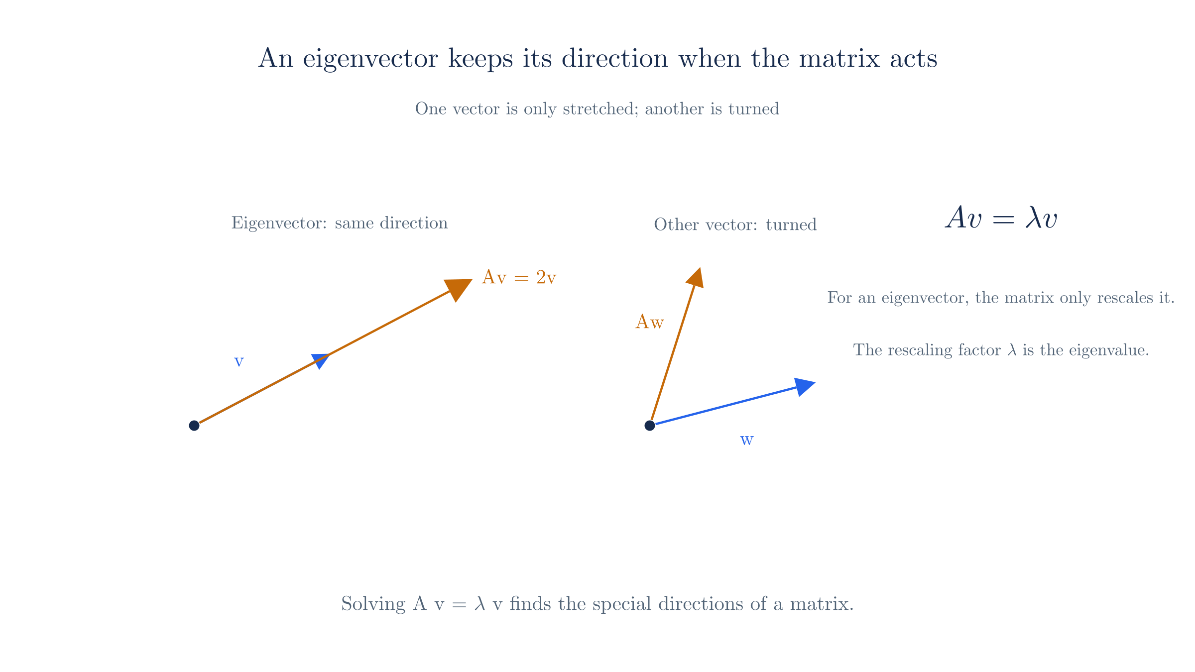
A matrix stretches an eigenvector without turning it, but turns an arbitrary vector.

5. Inner products and bra-ket notation

An inner product assigns a number to two vectors, measuring how much they overlap. For column vectors, it is the dot product with a conjugate:

$$⟨\mathbf{u}|\mathbf{v}⟩=u_1^{\ast }{v}_1+u_2^{\ast }{v}_2.$$

Its value is $\Vert \mathbf{v}{\Vert }^2=⟨\mathbf{v}|\mathbf{v}⟩$, the squared length, which is never negative.

Quantum mechanics abbreviates this with bra-ket notation. A ket $|\psi ⟩$ is a state vector; the matching bra $⟨\varphi |$ is the conjugate-transpose of a state vector, ready to form an inner product. The bracket $⟨\varphi |\psi ⟩$ is therefore the overlap of the two states. Inserting an operator between them,

$$⟨\varphi |\hat{A}|\psi ⟩,$$

means the overlap of $\varphi$ with the vector $\hat{A}|\psi ⟩$. The adjoint is defined so that moving an operator from one side to the other conjugates it:

$$⟨\varphi |{\hat{A}}^{†}\psi ⟩=⟨\hat{A}\varphi |\psi ⟩.$$

This notation first appears on First Quantization and is used from then on. A ket written as $|0⟩$ is a named state (the ground state or the vacuum), not the number zero.

6. Hermitian and unitary operators; trace

Two kinds of operator do most of the work:

• A Hermitian operator satisfies $\hat{A}={\hat{A}}^{†}$. Its eigenvalues are real, which is why observables are Hermitian. Eigenvectors with distinct eigenvalues are orthogonal.
• A unitary operator satisfies ${\hat{U}}^{†}\hat{U}=\hat{U}{\hat{U}}^{†}=1$. It preserves every inner product, so it maps normalized states to normalized states and describes time evolution and symmetry transformations.

For a Hermitian matrix we can always find a complete set of orthogonal eigenvectors. This is the spectral theorem: a state can be expanded in the eigenbasis of an observable, and the squared magnitudes of the expansion coefficients give outcome probabilities (First Quantization).

The trace of a square matrix is the sum of its diagonal entries, $\mathrm{tr}A={\sum }_i{A}_{ii}$. It appears when a closed fermion loop is evaluated, where the sum over the spinor index of a closed chain is a trace.

7. Changing basis

The components of a vector depend on the basis, but the vector itself does not. The same arrow has different coordinates when measured against a rotated pair of axes, yet it is still the same arrow.

The choice of basis is usually arbitrary, which is why it matters physically. An observer, or a reference frame, effectively picks a basis: two observers in relative motion pick different bases, but they describe the same particle. A law written in one basis must therefore hold in every other, because no observer's choice of coordinates is privileged.

That requirement sorts quantities into two kinds. A scalar has the same value in every basis, so it is an invariant, like the spacetime interval of relativity. A vector or tensor changes its components in a fixed, compensating way, and that rule is what makes quantities built from them come out invariant even while each component changes. Index notation and tensors develops these transformation rules, and Special Relativity is where they first become physical, because there the basis is a moving observer's frame.

Previous: Complex Numbers

Next: Index Notation and Tensors