Perturbation Theory: From the Lagrangian to the Feynman Rules

Adding an interaction to a quantum field theory leaves us with equations we cannot solve exactly. When the interaction is weak, we can approximate: expand the predicted amplitudes in powers of the coupling and keep the lowest nonzero terms. The Field Quantization page supplied the free fields and their particle states, and From Lagrangian to Experiment identified the S-matrix element as the quantity to calculate. This chapter expands that S-matrix in powers of the coupling. The Dyson series organizes the powers, and Wick's theorem organizes the field pairings within each term. The outcome is a short dictionary of factors — the Feynman rules that the next page assigns to each vertex and line in a diagram.

We will first use a real scalar field with a cubic interaction. It has no spin indices or gauge freedom, so we can follow the calculation before adding those features in QED. The optional Path Integrals sequence later gives a complementary derivation: Gaussian field integrals produce the same pairings and diagram rules.

We use natural units, $\hslash =c=1$, and metric $g_{\mu \nu }=\mathrm{diag}(1,-1,-1,-1)$. Setting $\hslash$ and $c$ to $1$ is a choice of units, not an approximation: energy, mass, and momentum share one unit, and distance is measured in units of time, so factors of $\hslash$ and $c$ drop out of the formulas. Thus $p^2=E^2-{\mathbf{p}}^2$. A physical free particle of mass $m$ is on shell, meaning $p^2=m^2$.

Outline of the argument

Each section develops one step of the calculation.

1. Define the interaction. Add $-g{\varphi }^3/3!$ to the free scalar Lagrangian.
2. Write the S-matrix. Solve the interaction-picture evolution equation as a time-ordered exponential, $S=T\exp [i\int d^{4}x{\mathcal{L}}_{\mathrm{int}}]$.
3. Expand in the coupling. The Dyson series groups contributions by their number of interaction factors.
4. Reorder the fields. Wick's theorem replaces time-ordered products with normal-ordered products and pair contractions.
5. Evaluate each contraction. The free-field expansion gives the propagator $i/(p^2-m^2+iϵ)$.
6. Assemble the amplitude. Attach the remaining fields to external particles, integrate over interaction positions, and count equivalent pairings.

We then apply the same method to QED, using its electron and photon fields.

The sums in this expansion arise from quantum evolution. Each term integrates over possible interaction positions and adds all operator pairings that connect the chosen initial and final states. We add amplitudes before calculating probabilities.

Two kinds of ordering enter. Time ordering places later operators on the left, as required by successive evolution. Normal ordering places creation operators on the left, which makes matrix elements easier to evaluate. Moving between these orders produces contractions, ordinary numerical factors associated with pairs of fields.

The setup: an interacting scalar

Begin with the free real scalar field from Field Quantization:

$${\mathcal{L}}_0=\frac{1}{2}({\partial }_{\mu }\varphi )({\partial }^{\mu }\varphi )-\frac{m^2}{2}{\varphi }^2.$$

Free quanta propagate without scattering. Add a cubic term to permit interactions:

$$\mathcal{L}={\mathcal{L}}_0-\frac{g}{3!}{\varphi }^3.$$

The coupling $g$ sets the interaction strength. The factor $3!$ will cancel the number of ways to assign three identical fields to a vertex's three legs.

This theory contains one spin-zero field, so all three legs belong to the same species. QED instead has a spinor $\psi$ and a vector $A_{\mu }$, with interaction $-q\bar{\psi }{\gamma }^{\mu }\psi A_{\mu }$. Both interactions contain three fields at one point, but QED has additional spin and polarization factors.

The cubic term makes the field equation nonlinear, as the interaction did in QED. We approximate amplitudes by expanding in small $g$. Here the cubic theory serves as a formal perturbative example; its potential alone has no stable global minimum.

The S-matrix as a series

In the interaction picture, field operators evolve with the free Hamiltonian, while states evolve with the interaction Hamiltonian. The S-matrix connects asymptotic incoming and outgoing free-particle states.

For this interaction, $H_{\mathrm{int}}=-\int d^{3}x{\mathcal{L}}_{\mathrm{int}}$. Solving the evolution equation gives

$$S=T\exp \left[i\int d^{4}x{\mathcal{L}}_{\mathrm{int}}(x)\right],$$

The symbol $T$ means time ordering: place later operators to the left^[1]. For two scalar fields, $T[\varphi (x)\varphi (y)]=\varphi (x)\varphi (y)$ if $x^0>y^0$, and $\varphi (y)\varphi (x)$ if $y^0>x^0$.

This ordering matters because field operators at different times generally do not commute. With ${\mathcal{L}}_{\mathrm{int}}=-g{\varphi }^3/3!$, expand the exponential as

$$S=\sum _{n=0}^{\infty }\frac{i^n}{n!}\int d^4{x}_1\cdots d^4{x}_{n}T[{\mathcal{L}}_{\mathrm{int}}(x_1)\cdots {\mathcal{L}}_{\mathrm{int}}(x_n)].$$

The term with $n$ interaction factors has order $g^n$ and integrates over $n$ spacetime positions. This is the Dyson series. The diagrams on the Feynman Rules page organize its terms.

To evaluate a term between particle states, we next rewrite its time-ordered field product using Wick's theorem.

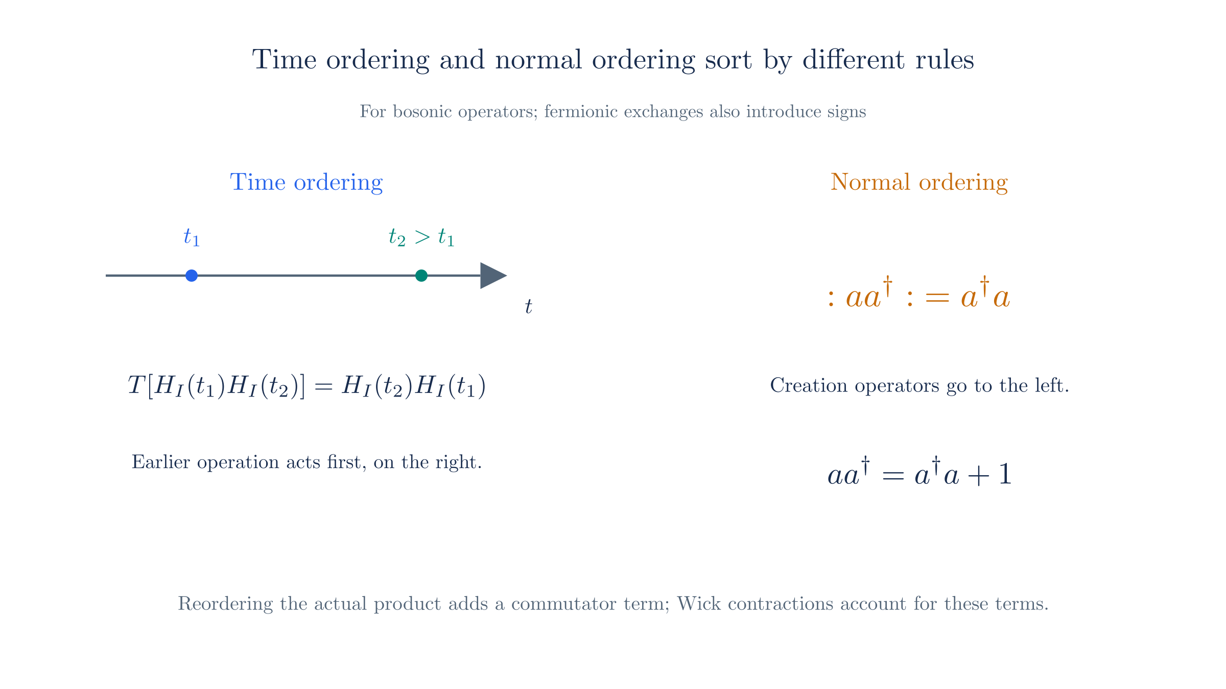
Time ordering places later interactions on the left. Normal ordering places creation operators on the left; commutators supply the extra terms.

Wick's theorem

The free-field expansion from Field Quantization has the form $\varphi ={\varphi }^{+}+{\varphi }^{-}$, where ${\varphi }^{+}$ annihilates and ${\varphi }^{-}$ creates a particle. Each part includes a plane-wave factor.

A normal-ordered product $:{\varphi }_1\cdots {\varphi }_n:$ places every creation operator to the left of every annihilation operator. This makes matrix elements easier to evaluate. An annihilation operator removes an incoming particle, or gives zero if none is available. A creation operator acting leftward on the vacuum bra also gives zero. The surviving terms contain the plane-wave factors associated with the external particles.

Time ordering sorts by time instead. To put a time-ordered product into normal order, we must sometimes commute an annihilation operator past a creation operator. Their nonzero commutator contributes an extra number. Wick's theorem accounts for all such terms.

For two free scalar fields, Wick's theorem states

$$T[\varphi (x)\varphi (y)]=:\varphi (x)\varphi (y):+⟨0|T[\varphi (x)\varphi (y)]|0⟩.$$

The second term is the contraction, a vacuum expectation value and therefore an ordinary number. We call this operation a contraction because it pairs two field operators and replaces the pair by one function, reducing the number of unpaired operators by two. For example,

$$\varphi (x)\varphi (y)⟶⟨0|T[\varphi (x)\varphi (y)]|0⟩={\Delta }_F(x-y).$$

This resembles contracting two tensor indices: two objects become linked and the result has fewer free parts. Here the resulting function is the propagator. It describes free propagation between $x$ and $y$, so a Feynman diagram represents the contraction by a line connecting those two interaction points.

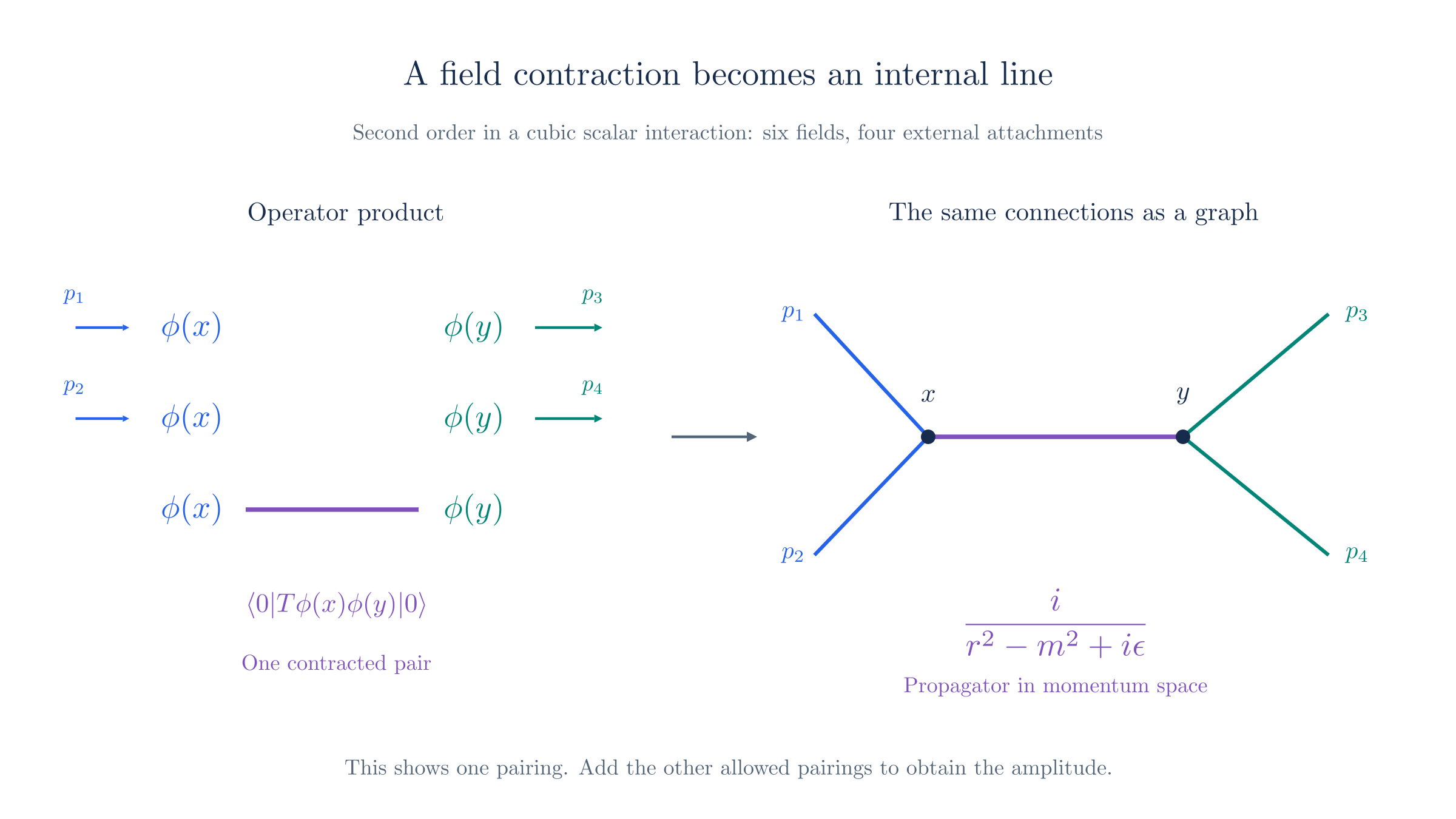
A contraction pairs two field operators and replaces them with a propagator. The Feynman diagram draws that propagator as the internal line between the vertices.

The vacuum also explains why complete contractions matter. Normal ordering places annihilation operators on the right, where they annihilate $|0⟩$, and creation operators on the left, where they annihilate $⟨0|$. A vacuum expectation value therefore vanishes if any field operator remains unpaired. Only terms in which contractions pair every field can contribute to a vacuum-to-vacuum expectation value.

Scattering matrix elements have external particle states rather than vacuum on both sides. In that case, some unpaired fields can annihilate incoming particles or create outgoing particles. A diagram draws these fields as external lines, while it draws contractions between interaction fields as internal propagator lines.

For a longer product, sum over every possible choice of disjoint contracted pairs. Leave all remaining fields in normal order, then evaluate them against the external states.

For a connected contribution with $k$ external particles, $k$ fields attach to those particles. At order $n$ in this cubic theory there are $3n$ fields, so the remaining $3n-k$ must contract in pairs. In particular, $3n-k$ must be even.

A three-leg contribution at first order has three fields and no internal contraction. A $2\to 2$ contribution at second order has six fields: four attach to the external particles and two contract into one internal line. We will evaluate both patterns below.

The propagator from the free field

The contraction can now be evaluated with the known free field. Including both time orderings and writing the result as one four-momentum integral gives

$$⟨0|T\varphi (x)\varphi (y)|0⟩=\int \frac{d^{4}p}{(2\pi {)}^4}\frac{i}{p^2-m^2+iϵ}{e}^{-ip\cdot (x-y)}.$$

The momentum-space factor appearing here is the propagator,

$$\frac{i}{p^2-m^2+iϵ}.$$

This is $i$ times the inverse of the free momentum-space quadratic operator $p^2-m^2$, with a specified boundary prescription: the denominator has poles near the mass-shell energies $p^0=\pm E_p$, and the $+iϵ$ shifts the positive-energy pole slightly below the real axis and the negative-energy pole slightly above it, implementing the Feynman time-ordering prescription. That is why the free Lagrangian determines the factor used between interaction vertices. An internal momentum need not be on shell.

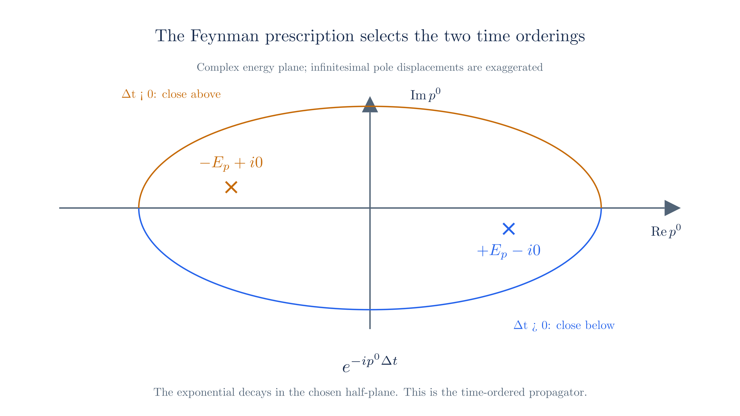
The positive-energy pole lies below the real axis and the negative-energy pole above it. The sign of the time separation determines which half-plane closes the contour.

The QED photon propagator

The QED page supplied the gauge-fixed photon field and its four formal polarization modes. We can now use the contraction machinery just developed to extract its internal-line factor:

$$D_{\mu \nu }(x-y)=⟨0|T{\hat{A}}_{\mu }(x){\hat{A}}_{\nu }(y)|0⟩.$$

Each mode contributes the massless scalar factor $i/(k^2+iϵ)$. Its polarization vectors supply the indices $\mu$ and $\nu$, while the indefinite-sign commutator supplies $-{\eta }_{\lambda }$:

$$D_{\mu \nu }(k)=\sum _{\lambda =0}^3(-{\eta }_{\lambda }){\epsilon }_{\mu }^{(\lambda )}{\epsilon }_{\nu }^{(\lambda )\ast }\frac{i}{k^2+iϵ}.$$

For the four-component basis used in QED,

$$\sum _{\lambda =0}^3{\eta }_{\lambda }{\epsilon }_{\mu }^{(\lambda )}{\epsilon }_{\nu }^{(\lambda )\ast }=g_{\mu \nu }.$$

Therefore, in Feynman gauge,

$$\boxed{D_{\mu \nu }(k)=\frac{-i{g}_{\mu \nu }}{k^2+iϵ}.}$$

The four components appear in this internal propagator because it belongs to the gauge-fixed formalism. Physical external photons still have only the two transverse polarizations. The internal momentum may be off shell, so it need not satisfy $k^2=0$.

Building amplitudes: the dictionary

Insert the Dyson series between the incoming and outgoing states. Apply Wick's theorem to each term. The surviving factors have three roles.

External lines. An uncontracted field annihilates an incoming particle with phase $e^{-ip\cdot x}$ or creates an outgoing particle with phase $e^{+ip\cdot x}$. A scalar has no spin or polarization index. After extracting the conventional external-state normalization, its external-line factor is $1$.

Internal lines. Each contracted pair contributes the free propagator, with momentum flowing between the two field positions.

Vertices. Each interaction factor contributes three fields and an integral over its position. Let $P$ be the signed sum of momenta entering that vertex. The plane waves give $\int d^{4}x{e}^{-ix\cdot P}=(2\pi {)}^4{\delta }^4(P)$, which enforces energy and momentum conservation there.

At a vertex, the $3!$ assignments of the identical fields cancel the $3!$ in ${\mathcal{L}}_{\mathrm{int}}$. The remaining vertex factor is $-ig$. Multiply it by a propagator $i/(p^2-m^2+iϵ)$ for each internal line, and integrate over momenta that conservation does not fix. Diagrams with equivalent pairings can also require symmetry factors.

Two low-order checks confirm the dictionary. Attaching three external particles to a single vertex gives the amplitude $i\mathcal{M}=-ig$. At second order in $2\to 2$ scattering, one contracted pair forms an internal line; the three distinct ways to route the external particles give three amplitudes of the same form, which add.

The resulting scalar rules are:

The product of these factors gives $i\mathcal{M}$, with any loop integrations and symmetry factors included. Enforce conservation at each vertex, then factor out the overall ${\delta }^4(P_f-P_i)$ according to From Lagrangian to Experiment^[4].

QED's rules are the same dictionary

For QED, we keep the method and change the fields: expand in the charge $q$ using ${\mathcal{L}}_{\mathrm{int}}=-q\bar{\psi }{\gamma }^{\mu }\psi A_{\mu }$. The Dyson series, contractions, and position integrals work as above. Fermionic reordering also introduces minus signs.

The free electron and photon fields determine their propagators and external-state factors. The interaction determines which fields meet at a vertex.

The electron propagator is $i(/r+m)/(r^2-m^2+iϵ)$, where $/r={\gamma }^{\mu }{r}_{\mu }$. In Feynman gauge, the photon propagator is $-i{g}_{\mu \nu }/(r^2+iϵ)$. Their matrix and vector indices reflect the fields they connect.

The interaction gives the vertex factor $-iq{\gamma }^{\mu }$. External electrons contribute $u(p)$ or $\bar{u}(p^{\prime })$, and external photons contribute polarization vectors ${\epsilon }_{\mu }(k)$ or their outgoing conjugates. These are the factors used on the Feynman Rules page.

The Field Quantization page derives the electron propagator. The QED page explains the photon’s gauge fixing, and the preceding section derives its propagator. With those free-field results, the expansion above produces the QED rules.

We set out to derive the diagram factors from the Lagrangian, and the expansion has now produced them: propagators come from the free terms, vertex factors from the interaction, and external factors from the particle states. The next page applies them to Compton scattering, then explains loop corrections and renormalization.