Quantum Electrodynamics

Two electrons that pass near each other come out moving in new directions. In quantum electrodynamics (QED) they scatter by exchanging a photon: one electron emits it and the other absorbs it, and neither the emission nor the absorption is seen directly. QED is the theory of the electron field, the photon field, and this coupling between them.

Two electrons scatter by exchanging a photon. The exchanged photon is internal: it is created and absorbed inside the process and never reaches a detector. Predicting how often the electrons deflect through a given angle needs a numerical factor for each vertex where the photon meets an electron line, and a factor for the internal photon line.

To turn a diagram like this into a number, we need a factor for each vertex and a factor for the internal photon line. This chapter derives the QED interaction and quantizes the photon field; Perturbation Theory extracts the propagator and assembles the diagram factors.

1. The vertex factor comes from an interaction term in the QED Lagrangian. Most of the chapter works out where that term comes from and why it has only one possible form.
2. The photon field supplies the internal-line factor. Quantizing it carries a complication the electron field did not: four potential components describe only two physical photons. The propagator is extracted later, after time ordering and contractions have been introduced.

A third QED building block, the propagator for an internal electron line, already came out of Field Quantization. It appears in processes such as Compton scattering rather than the exchange drawn above. The Perturbation Theory and Feynman Rules pages assemble all three factors into amplitudes.

We use natural units, $\hslash =c=1$, and metric $g_{\mu \nu }=\mathrm{diag}(1,-1,-1,-1)$, so $k^2=E_k^2-|\mathbf{k}{|}^2$.

The foundational distinction between spacetime labels and field-value spaces appears in Quantum Field Theory: Fields and Quanta §Spacetime, components, and value spaces. QED brings several of those objects together, so the following recap collects the notation used most often in this chapter.

The route to the interaction term runs through symmetry:

1. Assemble the free pieces. The Dirac and Maxwell Lagrangians describe the electron and photon fields propagating on their own.
2. Find the interaction. Requiring the theory to be unchanged by a local phase convention for the electron field forces a coupling to the photon potential.
3. Quantize the photon. The canonical construction needs a gauge-fixing step and a condition that picks out the physical states.
4. Extract the propagator. The quantized field supplies the factor for an internal photon line.

Recap of the Lagrangians

We begin with the two free Lagrangians from Action and Lagrangians.

The Dirac Lagrangian describes the free electron field:

$${\mathcal{L}}_{\text{Dirac}}=\bar{\psi }\left(i{\gamma }^{\mu }{\partial }_{\mu }-m\right)\psi .$$

Here $\psi$ is the electron's spinor field and $\bar{\psi }={\psi }^{†}{\gamma }^0$ is its Dirac adjoint. The derivative term describes propagation, and $-m\bar{\psi }\psi$ is the mass term. Applying the Euler–Lagrange equation gives the Dirac equation.

The Maxwell Lagrangian describes the free photon field. The potential $A_{\mu }$ has four components, and its derivatives form the electromagnetic field strength:

$${\mathcal{L}}_{\text{Maxwell}}=-\frac{1}{4}{F}_{\mu \nu }{F}^{\mu \nu },F_{\mu \nu }={\partial }_{\mu }{A}_{\nu }-{\partial }_{\nu }{A}_{\mu }.$$

Varying $A_{\mu }$ gives Maxwell's equations in free space, ${\partial }_{\mu }{F}^{\mu \nu }=0$.

Adding these two Lagrangians describes fields that propagate independently, with nothing passing between them. Electromagnetic scattering needs an interaction term as well. The next two sections show that requiring the electron Lagrangian to respect a local phase symmetry forces that term into one particular shape, the minimal coupling used in The Dirac Equation §1.

U(1) Global Symmetry

Multiplying the electron field by a constant phase changes no prediction. Take

$$\psi \to e^{i\alpha }\psi ,\bar{\psi }\to e^{-i\alpha }\bar{\psi },$$

with the same constant $\alpha$ everywhere. The probability density from First Quantization, $P={\psi }^{\ast }\psi$, is unchanged because the phase and its conjugate cancel. Relative phases between parts of a superposition still matter for interference; the transformation here rotates the whole field by one angle.

Every term in the free Dirac Lagrangian contains one $\psi$ and one $\bar{\psi }$. In the mass term the two phases cancel directly, $e^{-i\alpha }{e}^{i\alpha }=1$. In the kinetic term the constant phase passes through the derivative and then cancels the same way. The Lagrangian is therefore unchanged. A transformation that leaves the action unchanged is a symmetry, and this one is global because a single $\alpha$ applies across all of spacetime.

The symmetry also implies charge conservation. Noether's theorem attaches a conserved current to each continuous symmetry of the action, and for the phase transformation that current is

$$j^{\mu }=q\bar{\psi }{\gamma }^{\mu }\psi ,{\partial }_{\mu }{j}^{\mu }=0.$$

Its time component is the charge density and its spatial components describe charge flow. Integrating the density over all space gives the total electric charge, and the continuity equation says that charge moving between regions is never created or destroyed.

The phases $e^{i\alpha }$ form the group U(1). Each is a unitary $1\times 1$ matrix, equivalently a complex number of unit magnitude, and as $\alpha$ varies these numbers trace out the unit circle.

Local Gauge Symmetry U(1)

The phase of the electron field is not measurable on its own, so it is natural to ask that the theory not depend on this convention even when it is chosen separately at each point rather than once for all of spacetime. Replace the constant $\alpha$ by a function $\alpha (x)$:

$$\psi (x)\to e^{i\alpha (x)}\psi (x),\bar{\psi }(x)\to e^{-i\alpha (x)}\bar{\psi }(x).$$

The free Dirac Lagrangian does not survive this stronger demand. The mass term still cancels, because its two phase factors sit at the same point:

$$-m\bar{\psi }\psi \to -m{e}^{-i\alpha (x)}{e}^{i\alpha (x)}\bar{\psi }\psi =-m\bar{\psi }\psi .$$

The kinetic term does not. The derivative now acts on the phase as well as on $\psi$, and the product rule leaves an extra term proportional to $({\partial }_{\mu }\alpha )\bar{\psi }{\gamma }^{\mu }\psi$, which does not vanish for a general $\alpha (x)$.

To cancel the extra term, introduce a field that shifts under the same transformation. Give the vector potential the rule

$$A_{\mu }\to A_{\mu }-\frac{1}{q}{\partial }_{\mu }\alpha ,$$

and fold it into the derivative:

$$D_{\mu }={\partial }_{\mu }+iq{A}_{\mu }.$$

The shift in $A_{\mu }$ places $-i{\partial }_{\mu }\alpha$ inside $D_{\mu }$, which cancels the $+i{\partial }_{\mu }\alpha$ from differentiating the phase. What remains is

$$D_{\mu }\psi \to e^{i\alpha (x)}{D}_{\mu }\psi ,$$

so $D_{\mu }\psi$ carries the same phase as $\psi$ itself. That is why $D_{\mu }$ is called the covariant derivative. Multiplying by $\bar{\psi }$ removes the phase, and the kinetic term built from $D_{\mu }$ is locally invariant.

Expanding it,

$$\bar{\psi }i{\gamma }^{\mu }{D}_{\mu }\psi =\bar{\psi }i{\gamma }^{\mu }{\partial }_{\mu }\psi -q\bar{\psi }{\gamma }^{\mu }\psi A_{\mu },$$

produces exactly one interaction term, coupling the electron current $j^{\mu }=q\bar{\psi }{\gamma }^{\mu }\psi$ to the potential $A_{\mu }$. Local U(1) invariance fixes its form. The charge $q$ sets its strength, and the symmetry argument does not predict the numerical value.

The photon potential now appears in the electron's dynamics. The next section adds a kinetic term for $A_{\mu }$ so that electromagnetic disturbances can propagate on their own.

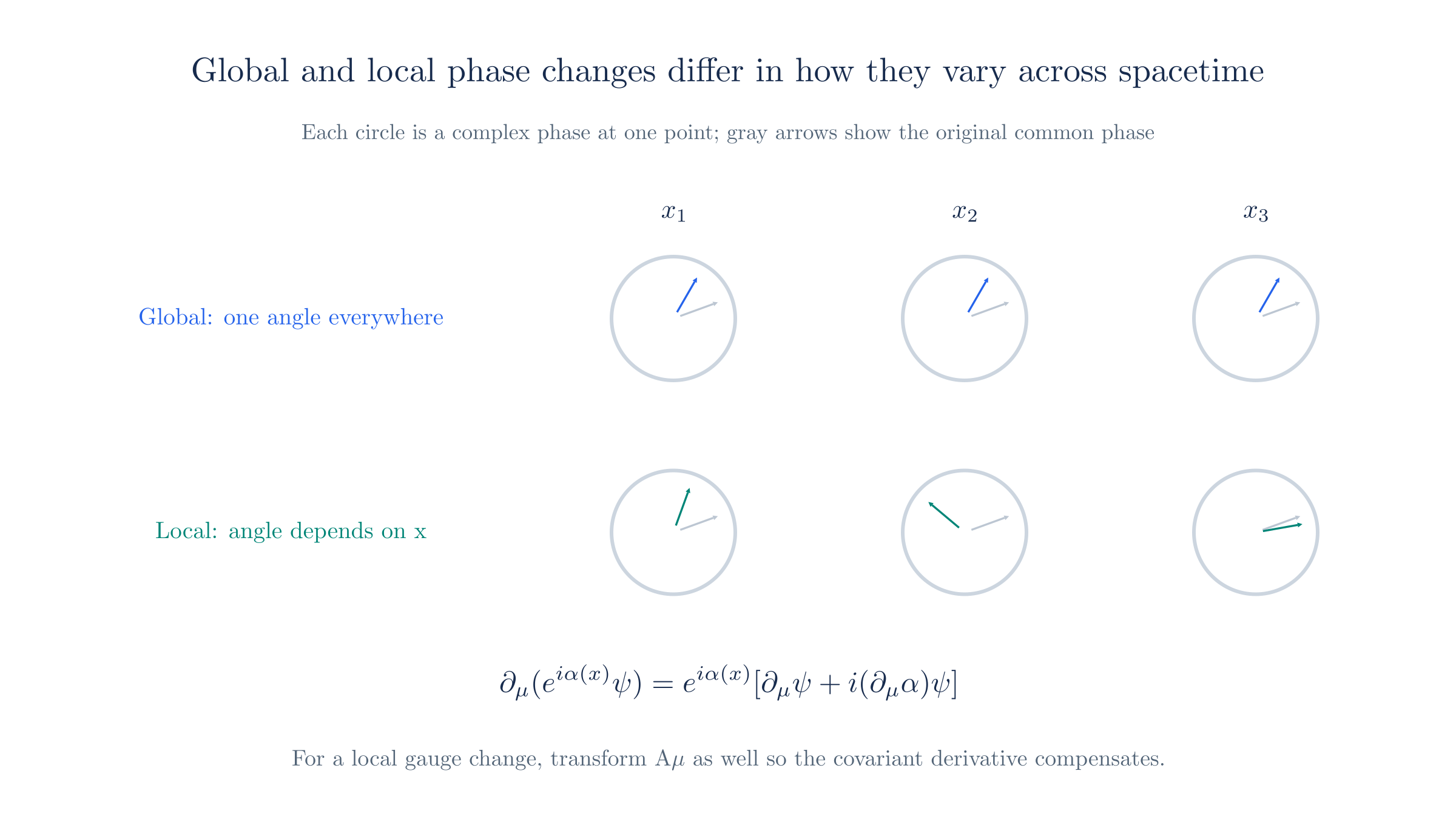
A global phase rotation uses one angle everywhere. A local rotation has a position-dependent angle, whose derivative requires a compensating transformation of the gauge potential.

QED Lagrangian

The potential $A_{\mu }$ now belongs to the same locally gauge-invariant theory as the electron field. Its kinetic term must therefore be the same kinetic term for two gauge-equivalent potentials. We do not modify the kinetic term itself: we transform $A_{\mu }$, then check that the existing Maxwell term is unchanged. The field strength here is the same $F_{\mu \nu }$ introduced in the free Maxwell theory. Write

$$A_{\mu }^{\prime }=A_{\mu }-\frac{1}{q}{\partial }_{\mu }\alpha .$$

Substitute this transformed potential into the same definition:

$$F_{\mu \nu }={\partial }_{\mu }{A}_{\nu }-{\partial }_{\nu }{A}_{\mu }$$

$$\begin{array}{rl}{F}_{\mu \nu }^{\prime }& ={\partial }_{\mu }{A}_{\nu }^{\prime }-{\partial }_{\nu }{A}_{\mu }^{\prime }\\ & =F_{\mu \nu }-\frac{1}{q}\left({\partial }_{\mu }{\partial }_{\nu }\alpha -{\partial }_{\nu }{\partial }_{\mu }\alpha \right)\\ & =F_{\mu \nu }.\end{array}$$

The added piece vanishes because mixed partial derivatives commute. Thus the transformation changes the potential's description but not the electromagnetic field strength.

The Maxwell term $-\frac{1}{4}{F}_{\mu \nu }{F}^{\mu \nu }$ is therefore gauge invariant. It is the standard Lorentz-invariant term quadratic in the field strength. Gauge symmetry permits additional higher-order terms in an effective theory, so it constrains the Lagrangian rather than fixing it uniquely.

Combining the photon term with the covariant Dirac term,

$${\mathcal{L}}_{\text{QED}}=-\frac{1}{4}{F}_{\mu \nu }{F}^{\mu \nu }+\bar{\psi }\left(i{\gamma }^{\mu }{D}_{\mu }-m\right)\psi ,D_{\mu }={\partial }_{\mu }+iq{A}_{\mu }.$$

Expanding the covariant derivative separates the three contributions:

$${\mathcal{L}}_{\text{QED}}=-\frac{1}{4}{F}_{\mu \nu }{F}^{\mu \nu }+\bar{\psi }\left(i{\gamma }^{\mu }{\partial }_{\mu }-m\right)\psi -q\bar{\psi }{\gamma }^{\mu }\psi A_{\mu }.$$

They describe photon propagation, free electron propagation, and the electron–photon interaction.

The interaction term is the source of the vertex factor promised in the introduction. Stripping the three fields off $-q\bar{\psi }{\gamma }^{\mu }\psi A_{\mu }$ and keeping the factor of $i$ from the S-matrix expansion leaves

$$-iq{\gamma }^{\mu },$$

the number attached to each point where a photon line meets an electron line. The Feynman Rules page derives this in full.

A direct photon mass term proportional to $m_{\gamma }^2{A}_{\mu }{A}^{\mu }$ is not gauge invariant, because $A_{\mu }{A}^{\mu }$ changes under the gradient shift. An unbroken U(1) gauge symmetry therefore forbids it, and the photon we quantize next is massless.

Quantizing the Photon Field

The photon propagator is the factor for an internal photon line. The Field Quantization page built propagators by expanding a free field into modes and treating each mode as an oscillator. The photon follows the same route with one extra step: the four components of $A_{\mu }$ carry only two physical polarizations, and the construction has to remove the other two.

On a first read, take two results from this section and move on. The photon has two physical polarizations, and its propagator in Feynman gauge is

$$D_{\mu \nu }(k)=\frac{-i{g}_{\mu \nu }}{k^2+iϵ}.$$

The rest of the section works through the steps needed to reach it.

The plan is to make all four components easy to quantize, then restrict the quantum states so that only the two physical polarizations survive. We first see where the two come from, then why the direct canonical construction stalls.

Counting a free photon's polarizations

Write the potential as a single plane wave,

$$A^{\mu }(x)={\epsilon }^{\mu }{e}^{-ik\cdot x},$$

where $k^{\mu }=(E_k,\mathbf{k})$ sets the energy and momentum and the polarization vector ${\epsilon }^{\mu }$ sets the amplitude of each component of the potential. A complex wave keeps the algebra short; its real part is the physical classical field.

Putting this wave into the free Maxwell equation ${\partial }_{\mu }{F}^{\mu \nu }=0$ leaves one condition on the momentum and polarization,

$$k^2{\epsilon }^{\nu }=k^{\nu }(k\cdot \epsilon ).\text{\hspace{1em}(1)}$$

It has two consequences. First, a wave that carries a nonzero electromagnetic field must have $k^2=0$, the massless energy–momentum relation $E_k=|\mathbf{k}|$, because a polarization proportional to $k$ produces a vanishing field strength. Such a potential oscillates without any $\mathbf{E}$ or $\mathbf{B}$ and is called pure gauge. Second, with $k^2=0$ the condition becomes $k\cdot \epsilon =0$, which ties the four amplitude components together and removes one of them.

Gauge freedom removes one more amplitude. A gauge transformation shifts the potential by a gradient,

$$A_{\mu }⟶A_{\mu }+{\partial }_{\mu }\chi ,$$

which leaves $F_{\mu \nu }$ unchanged because the extra term is ${\partial }_{\mu }{\partial }_{\nu }\chi -{\partial }_{\nu }{\partial }_{\mu }\chi =0$. For a gauge function with the same plane-wave dependence, the gradient is proportional to $k_{\mu }$, so the polarization shifts as ${\epsilon }^{\mu }\to {\epsilon }^{\mu }+\alpha k^{\mu }$. Choosing $\alpha$ appropriately removes the remaining non-transverse amplitude. Only the two directions perpendicular to the motion remain as independent physical polarizations:

$${\epsilon }^{(1)}=(0,1,0,0),{\epsilon }^{(2)}=(0,0,1,0).$$

For a free photon, the count is therefore four potential components, minus one Maxwell constraint, minus one gauge freedom, leaving two physical polarizations.

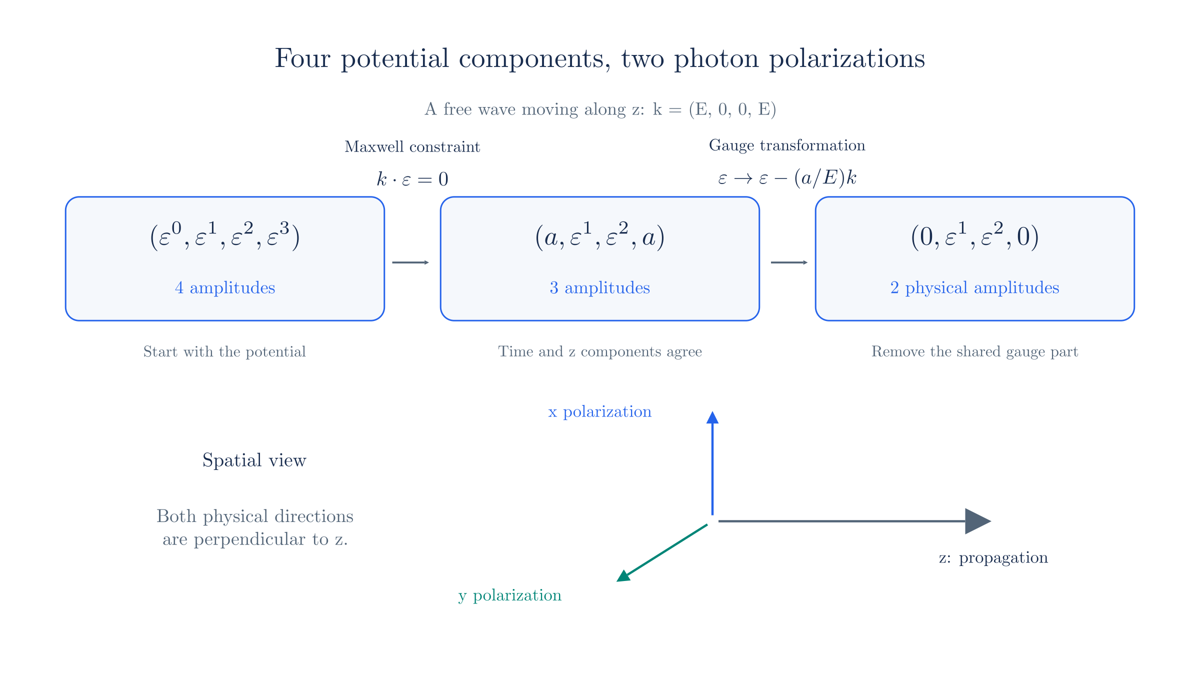
A photon moving along z: the Maxwell constraint ties the time and z components together, and a gauge transformation removes that shared component, leaving two transverse polarizations.

Why the canonical construction stalls

Canonical quantization pairs each field with a conjugate momentum. For each component of the potential, calculate

$${\pi }^{\mu }=\frac{\partial \mathcal{L}}{\partial ({\partial }_0{A}_{\mu })}=-F^{0\mu }.$$

The spatial components come out as ${\pi }^i=E^i$. The time component does not: antisymmetry forces $F^{00}=0$, so

$${\pi }^0=0.$$

The same gap shows up directly in the Lagrangian, where ${\dot{A}}_0$ never appears, because the time derivatives in $F_{\mu \nu }$ act only on the spatial components of the potential.

A vanishing conjugate momentum blocks the usual canonical commutator. The standard relation for $A_0$ would set the right-hand delta function equal to zero, which cannot hold. The vanishing momentum instead marks $A_0$ as a constrained variable. Its Maxwell equation is Gauss's law, $\nabla \cdot \mathbf{E}=0$, a condition on the electric field at one instant with no time derivative to carry it to the next. In the Hamiltonian description, $A_0$ enforces that constraint.

Constrained systems can still be quantized. We use a method that keeps Lorentz covariance visible: add a gauge-fixing term that gives all four components a nonzero conjugate momentum, quantize, then select the physical states afterward.

Fixing the gauge

Despite its name, gauge fixing does not mean adding another field to the gauge potential. These are two different operations:

• A gauge transformation changes the potential, $A_{\mu }\to A_{\mu }+{\partial }_{\mu }\chi$, without changing $F_{\mu \nu }$.
• Gauge fixing leaves $A_{\mu }$ as the field variable and adds a term ${\mathcal{L}}_{\text{gf}}$ to the QED Lagrangian. The term controls the redundant gauge freedom so that the field can be quantized covariantly.

Thus it is the Lagrangian, not the potential, that is modified:

$$\boxed{{\mathcal{L}}_{\text{QED}}⟶{\mathcal{L}}_{\text{QED}}^{(\xi )}={\mathcal{L}}_{\text{QED}}+{\mathcal{L}}_{\text{gf}}}$$

The gauge freedom lets many potentials describe the same $\mathbf{E}$ and $\mathbf{B}$. A useful choice is the Lorenz condition,^[1]

$${\partial }_{\mu }{A}^{\mu }=0.$$

The contraction makes this condition Lorentz covariant: it has the same form in every Lorentz frame.

To see how we can reach it, apply a gauge transformation. The divergence changes as

$$\partial \cdot A⟶\partial \cdot A+\square \chi ,\square ={\partial }_t^2-{\nabla }^2.$$

Choosing $\chi$ to solve

$$\square \chi =-\partial \cdot A$$

therefore gives a potential satisfying the Lorenz condition, with suitable boundary conditions in the flat spacetime setting used here. Some freedom remains: a further transformation with $\square \chi =0$ preserves the condition. For plane waves, this includes the shift along $k$ that we used to remove the amplitude $a$.

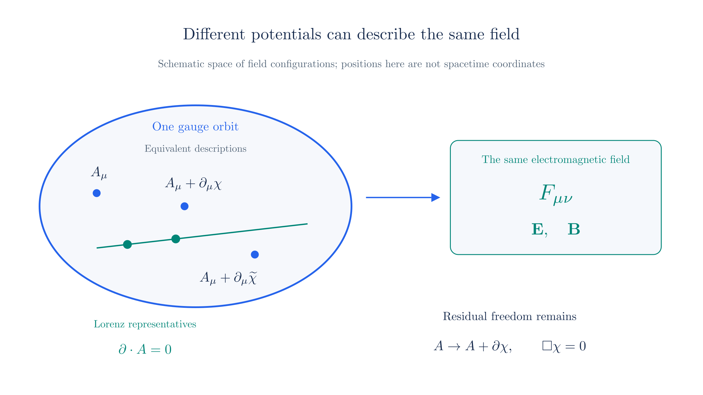
Equivalent potentials belong to one gauge orbit and produce the same electromagnetic field. The Lorenz condition still permits residual gauge transformations.

In the quantum theory, this cannot become an exact identity between independent canonical field operators. The divergence contains ${\dot{\hat{A}}}^0$, which will be related to the momentum of ${\hat{A}}_0$. Setting that divergence identically to zero conflicts with the canonical commutator.^[2] We will instead impose a weaker condition on physical states.

The name gauge fixing refers to controlling which representatives of each gauge-equivalence class occur in the calculation. It does not mean fixing or repairing the gauge field $A_{\mu }$ itself. The term is not unique. A Lorentz-covariant family is

$${\mathcal{L}}_{\text{gf}}=-\frac{1}{2\xi }({\partial }_{\mu }{A}^{\mu }{)}^2.$$

Different values of $\xi$ give different intermediate propagators and different treatments of the unphysical gauge directions. We choose $\xi =1$, called Feynman gauge, because it makes the four components decouple and gives the simplest canonical quantization. This is a choice of formalism, not a new physical interaction.

For this choice, to make the canonical construction possible, add the following term to ${\mathcal{L}}_{\text{QED}}$:

$${\mathcal{L}}_{\text{gf}}=-\frac{1}{2}({\partial }_{\mu }{A}^{\mu }{)}^2.$$

Since

$$\partial \cdot A={\dot{A}}^0+\nabla \cdot \mathbf{A},$$

the added term contains $-\frac{1}{2}({\dot{A}}^0{)}^2$. The missing velocity now appears, and the momentum becomes

$${\pi }^0=-\partial \cdot A.$$

We have made all four components dynamical. This enlarges the space of solutions we quantize, so adding the term and selecting physical states must go together. The fact that the term vanishes on Lorenz-obeying fields is not, by itself, a proof that the quantum predictions stay the same. The Gupta–Bleuler condition below removes the extra gauge-sector states; equivalently, in other quantization formalisms, Ward identities or BRST symmetry ensure that gauge-invariant observables do not depend on $\xi$.

An arbitrary extra term would change the physical equations and could change the predictions. Gauge fixing is special because the original Maxwell action is constant along gauge orbits: all potentials $A_{\mu }+{\partial }_{\mu }\chi$ in one orbit describe the same physical field. The gauge-fixing term changes which representative is selected and adds motion in the redundant directions, but it does not remove the physical gauge-equivalence class. In a path integral, it changes the weighting of descriptions within each orbit; the physical-state restriction (or, in another formalism, the corresponding gauge-fixing determinant/BRST construction) removes that artificial change from gauge-invariant predictions.

The added term also decouples the components: inside the action, the component-mixing part of the Maxwell term cancels against the gauge-fixing term after two integrations by parts. The equivalent Lagrangian is

$$\boxed{\mathcal{L}=-\frac{1}{2}({\partial }_{\mu }{A}_{\nu })({\partial }^{\mu }{A}^{\nu }).}$$

For this form of the Lagrangian, the canonical momenta are

$${\pi }^{\nu }=-{\partial }^0{A}^{\nu },{\pi }^0=-{\dot{A}}^0.$$

The last expression differs from the momentum before integration by parts because changing the boundary terms can change the canonical momenta. Both Lagrangians give the same bulk equations of motion.

Each component now obeys a massless wave equation,

$$\square A_{\nu }=0.$$

This choice gives four decoupled wave equations, which we can quantize using the oscillator construction. We still need to recover the two-polarization physical state space.

Quantizing the gauge-fixed field

With the components decoupled, expand the field into four families of modes. For momentum along $z$, choose the polarization basis

$${\epsilon }^{(0)}=(1,0,0,0),{\epsilon }^{(1)}=(0,1,0,0),$$

$${\epsilon }^{(2)}=(0,0,1,0),{\epsilon }^{(3)}=(0,0,0,1).$$

The labels $1$ and $2$ are the transverse directions. The label $0$ is timelike, and $3$ is longitudinal, pointing along the spatial momentum. Promote each mode amplitude to an annihilation operator and its complex conjugate to a creation operator:

$${\hat{A}}_{\mu }(x)=\int \frac{d^{3}k}{(2\pi {)}^3}\frac{1}{\sqrt{2E_k}}\sum _{\lambda =0}^3\left[{\hat{c}}_{\lambda }(k){\epsilon }_{\mu }^{(\lambda )}(k)e^{-ik\cdot x}+{\hat{c}}_{\lambda }^{†}(k){\epsilon }_{\mu }^{(\lambda )\ast }(k)e^{+ik\cdot x}\right],E_k=|\mathbf{k}|.$$

This has the same structure as the scalar field expansion. The extra sum accounts for the four polarization directions. Each ${\hat{c}}_{\lambda }$ removes a quantum in its mode, and each ${\hat{c}}_{\lambda }^{†}$ adds one.

At this stage, these operators build an auxiliary state space, not yet the physical photon space. For one momentum, a general candidate one-quantum state has the form

$$|\Psi ⟩=\sum _{\lambda =0}^3{z}_{\lambda }{\hat{c}}_{\lambda }^{†}(k)|0⟩.$$

The coefficients $z_{\lambda }$ can initially include all four polarizations. The timelike mode is the awkward one. The metric gives the time component a kinetic term of the opposite sign from the three spatial components, and a single timelike quantum comes out with negative norm. We therefore need a test that distinguishes acceptable candidates from the extra states introduced by the gauge-fixed construction.

The Gupta–Bleuler condition supplies that test. Apply the annihilation part of the Lorenz condition to a candidate state:

$$\boxed{({\partial }_{\mu }{\hat{A}}^{\mu }{)}^{(+)}|\Psi ⟩=0.}$$

The superscript $(+)$ keeps the positive-frequency terms, which contain ${\hat{c}}_{\lambda }{e}^{-ik\cdot x}$. A candidate that satisfies this equation belongs to the physical subspace; only then do we call it a physical state. For a one-photon candidate, the test reduces to $k\cdot z=0$, the same polarization constraint that follows from Maxwell's equation.

For momentum along $z$, the condition ties the timelike and longitudinal modes together so their contributions to observable quantities cancel. States that differ only by a zero-norm gauge mode then represent the same physical state. After this identification, the independent states contain only the two transverse polarizations.

An external photon in a scattering calculation therefore carries one of these two polarizations, or a superposition of them such as circular polarization.

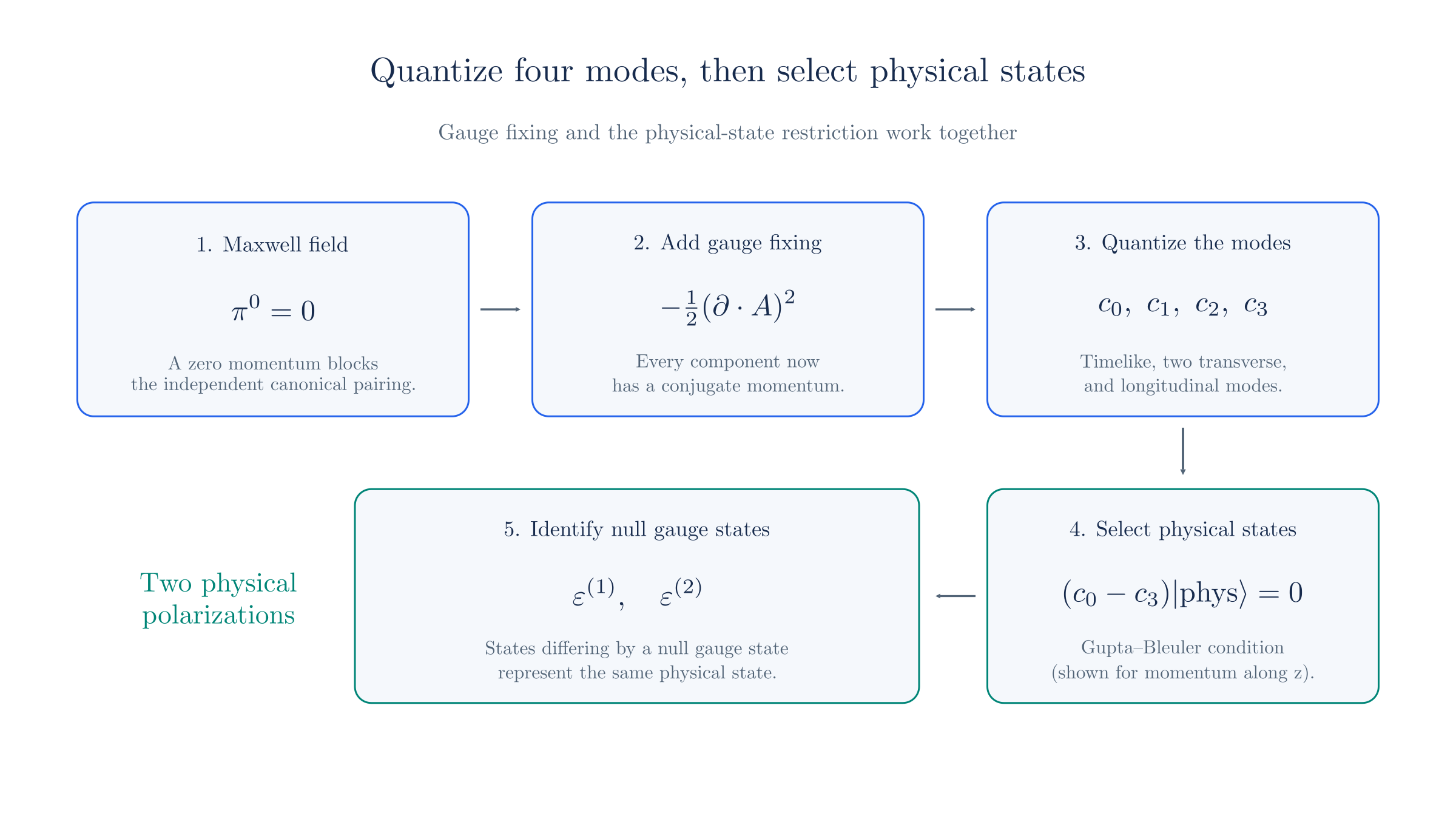
Gauge fixing gives four quantizable modes. The physical-state condition and identification of null gauge states recover the two physical photon polarizations.

Handoff to perturbation theory

The photon field is now quantized, including its gauge fixing and physical-state restriction. The next step is to introduce time ordering and contractions, then extract the photon propagator from this field. Perturbation Theory performs that extraction and assembles the QED factors into amplitudes. The Feynman Rules page then uses those factors in scattering calculations, and From Lagrangian to Experiment connects the resulting amplitude to measured rates.