Higgs Mechanism

In Electroweak Unification, we identified the photon, $W^{\pm }$, and $Z$ and related their interactions. Their masses remained unexplained. Direct gauge-boson mass terms would violate the electroweak gauge symmetry, while an electron mass term joins left- and right-chiral fields with different electroweak charges.

We now introduce a scalar field whose lowest-energy value is nonzero. Interactions with that vacuum value produce mass terms when we expand around the ground state, even though the original Lagrangian respects the full gauge symmetry. These are different from explicit mass terms inserted directly into the Lagrangian: the mass terms here emerge from already-invariant interactions after the field is expanded around its vacuum value. Fluctuations about the vacuum describe an additional particle, the Higgs boson. The field's vacuum value and the particle excitation play different roles; we will distinguish them throughout.

We use natural units, $\hslash =c=1$, the metric $(+,-,-,-)$, and the covariant-derivative conventions of the previous two chapters. The mass formulas below are at tree level, before quantum corrections.

The steps connect as follows:

1. Separate the symmetry of the laws from the symmetry of the ground state. A potential can respect a symmetry while its lowest-energy configurations do not. Selecting one of those configurations is spontaneous symmetry breaking.
2. Gauge the broken symmetry in the simplest case. A charged scalar with a nonzero vacuum value gives a $U(1)$ gauge field a mass. This simpler example shows how the scalar phase becomes the additional polarization of a massive vector.
3. Apply the construction to $SU(2{)}_L\times U(1{)}_Y$. A scalar doublet with a suitable potential acquires a vacuum value that leaves electric charge unbroken.
4. Read off the fermion masses. Coupling that doublet to the fermions gives each charged fermion a mass set by its coupling strength.
5. Read off the gauge-boson masses. Expanding the doublet's kinetic term gives masses to the $W$ and $Z$ while leaving the photon massless.

Spontaneous Symmetry Breaking

A symmetric law can have a ground state that does not share its symmetry. Consider an idealized magnet whose spin interactions have no preferred direction. Below its critical temperature, its magnetization points in one direction, although other orientations have the same energy. We will construct a field with an analogous set of lowest-energy configurations, then study small disturbances around one of them.

Take a single complex scalar field $\varphi (x)$ with a global $U(1)$ symmetry, $\varphi \to e^{i\alpha }\varphi$ (see the appendix on groups for $U(1)$). Its Lagrangian is

$$\mathcal{L}={\partial }_{\mu }{\varphi }^{\ast }{\partial }^{\mu }\varphi -V(\varphi ),V(\varphi )=-{\mu }^2{\varphi }^{\ast }\varphi +\lambda ({\varphi }^{\ast }\varphi {)}^2,$$

with ${\mu }^2>0$ and $\lambda >0$. The phase rotation leaves ${\varphi }^{\ast }\varphi$ unchanged, so $\mathcal{L}$ is invariant. The unusual part is the sign of the quadratic term. A positive ${\mu }^2$ in front of $-{\varphi }^{\ast }\varphi$ means the field configuration $\varphi =0$ sits at a local maximum of $V$, not a minimum.

The vacuum is the lowest-energy state. At the classical level, we find the corresponding vacuum field configuration by minimizing the potential. For a static, spatially uniform scalar field, derivative contributions to the energy vanish, so we minimize $V$. To find the minima, write ${\varphi }^{\ast }\varphi ={\rho }^2$ and minimize $V=-{\mu }^2{\rho }^2+\lambda {\rho }^4$. Treating $r={\rho }^2$ as the variable gives $dV/dr=-{\mu }^2+2\lambda r=0$, hence

$${\varphi }^{\ast }\varphi =\frac{{\mu }^2}{2\lambda }\equiv \frac{v^2}{2}.$$

The minimum is not a point but a circle in the complex plane: every $\varphi$ with $|\varphi |=v/\sqrt{2}$ has the same lowest energy. We use $v$ to parameterize the vacuum expectation value, the value of the field in the ground state; with our normalization, its magnitude is $v/\sqrt{2}$. The vacuum state means the lowest-energy state, not a state in which the field must have value zero. We describe particles as excitations above that ground state. Choose the real point on the circle,

$$⟨\varphi ⟩=\frac{v}{\sqrt{2}},$$

taking the vacuum value real. The Lagrangian's $U(1)$ symmetry still holds, but this vacuum is not invariant under it: a phase rotation moves it to a different point on the circle. A symmetry of the Lagrangian that the chosen vacuum does not share is spontaneously broken. The potential still has the symmetry. The nonzero vacuum value specifies which member of the equal-energy, or degenerate, set we expand around.

For the ideal uniform vacuum, this same minimum is chosen at every spacetime point, so $\varphi (x)=v/\sqrt{2}$ is constant. Different choices around the circle describe different possible vacuum orientations; fluctuations around the chosen one are treated separately.

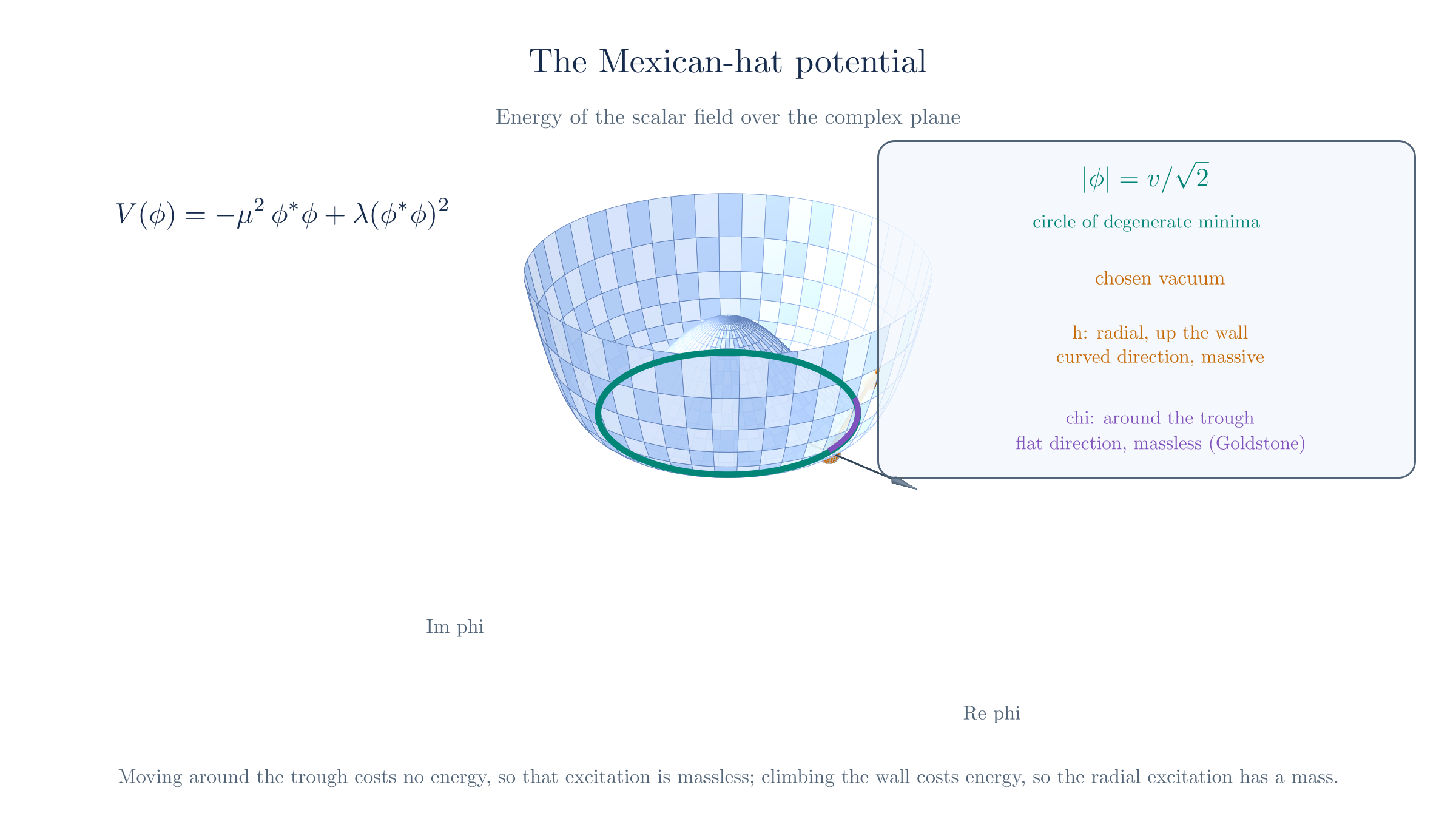
The two independent excitations above this vacuum behave differently. Write the field as a fluctuation about the chosen point,

$$\varphi (x)=\frac{1}{\sqrt{2}}(v+h(x)+i\chi (x)),$$

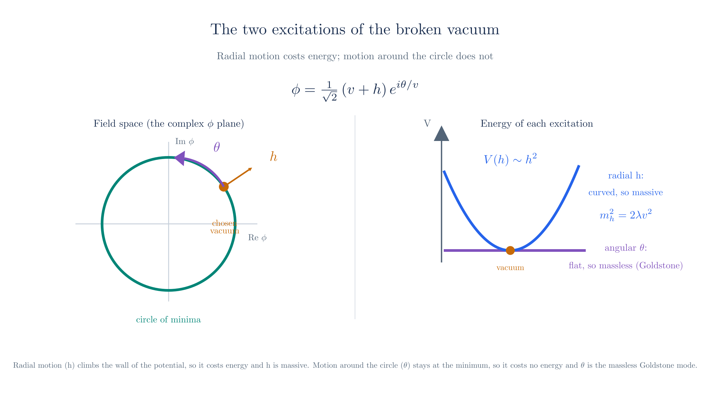
The real fields $h$ and $\chi$ describe small displacements in the radial and tangential directions at the chosen vacuum. At first order, $\chi$ changes the phase; a finite displacement around the circle is more accurately described with polar coordinates below.

The terms quadratic in these fluctuations determine their free propagation:

$${\mathcal{L}}_{\mathrm{quadratic}}=\frac{1}{2}{\partial }_{\mu }h{\partial }^{\mu }h+\frac{1}{2}{\partial }_{\mu }\chi {\partial }^{\mu }\chi -\frac{1}{2}{m}_h^2{h}^2,m_h^2=2\lambda v^2,m_{\chi }^2=0.$$

For a canonically normalized scalar, $\frac{1}{2}(\partial f{)}^2-\frac{1}{2}{m}^2{f}^2$ gives $(\square +m^2)f=0$, hence $E^2={\mathbf{p}}^2+m^2$. This is why the quadratic coefficient identifies a particle mass. Higher powers describe interactions between the excitations.

The massless field $\chi$ is a Goldstone boson. Its absence of mass is not a coincidence of this potential: moving along the circle of minima costs no energy, because every point on the circle is a degenerate vacuum, and a field excitation that costs no energy at long wavelength has no mass. For relativistic scalar theories of this kind, Goldstone's theorem gives one massless mode per broken continuous global generator. We state the general theorem without proof because its derivation requires a longer discussion of conserved currents; the expansion above proves the result for this example. Spatially varying phase disturbances still carry gradient energy; masslessness means zero rest energy, not zero energy for every wave. The massive field $h$ measures excursions in the direction that does cost energy, out of the trough and up the wall of the potential.

The electroweak symmetry is local, so the global-symmetry result is not yet our final particle spectrum. The next step shows why the phase does not remain an independent massless particle when a gauge field is present.

Higgs Mechanism U(1)

Now make the $U(1)$ local, exactly as QED makes the electron's phase symmetry local. Promoting $\varphi \to e^{i\alpha (x)}\varphi$ to a spacetime-dependent phase requires a gauge field $A_{\mu }$ and the covariant derivative $D_{\mu }={\partial }_{\mu }+iq{A}_{\mu }$, with $q$ the scalar's gauge coupling, taken positive here. This $A_{\mu }$ belongs to a toy model; it is not the physical photon of the electroweak theory. The Lagrangian becomes

$$\mathcal{L}=(D_{\mu }\varphi {)}^{\ast }(D^{\mu }\varphi )-V(\varphi )-\frac{1}{4}{F}_{\mu \nu }{F}^{\mu \nu },$$

with the same potential as before and the same circle of minima. The field strength $F_{\mu \nu }={\partial }_{\mu }{A}_{\nu }-{\partial }_{\nu }{A}_{\mu }$ describes the free gauge field, which is massless on its own, as a photon-like mass term would break the gauge symmetry.

Unlike a global phase change, a gauge transformation changes both $\varphi$ and $A_{\mu }$ as two parts of the same description. Near the nonzero vacuum, we can choose the scalar to be real at each point, provided we transform the gauge field at the same time. This choice is unitary gauge:

$$\varphi (x)=\frac{1}{\sqrt{2}}(v+h(x)).$$

The phase no longer appears as a separate scalar field. Its dynamical degree of freedom remains in the gauge field, which will now have three physical polarizations rather than two. Gauge fixing does not discard a physical mode.

Proca equation for the massive vector

The scalar vacuum has now supplied a vector mass, $m_A=qv$. To find how this massive field propagates, keep the terms quadratic in $A_{\mu }$ and set aside its interactions with the Higgs fluctuation $h$. In unitary gauge, the free vector Lagrangian is

$${\mathcal{L}}_{\mathrm{free}}=-\frac{1}{4}{F}_{\mu \nu }{F}^{\mu \nu }+\frac{1}{2}{m}_A^2{A}_{\mu }{A}^{\mu }.$$

The mass here comes from the original gauge-invariant scalar kinetic term. We have reached this Lagrangian after expanding around the nonzero vacuum, rather than inserting a mass into the unbroken gauge theory.

Vary the vector field. The Maxwell calculation in Action and Lagrangians already gives the derivative with respect to ${\partial }_{\mu }{A}_{\nu }$. The new mass term also contributes a derivative with respect to $A_{\nu }$:

$$\frac{\partial {\mathcal{L}}_{\mathrm{free}}}{\partial ({\partial }_{\mu }{A}_{\nu })}=-F^{\mu \nu },\frac{\partial {\mathcal{L}}_{\mathrm{free}}}{\partial A_{\nu }}=m_A^2{A}^{\nu }.$$

The factor $\frac{1}{2}$ cancels the two contributions from differentiating $A_{\rho }{A}^{\rho }$. Substituting into the Euler–Lagrange equation gives

$$-{\partial }_{\mu }{F}^{\mu \nu }-m_A^2{A}^{\nu }=0,\boxed{{\partial }_{\mu }{F}^{\mu \nu }+m_A^2{A}^{\nu }=0.}$$

This is the Proca equation, the free equation for a massive spin-1 field. Maxwell describes the massless vector; Proca describes the massive vector we have obtained through Higgs.

Derive the constraint. Take the divergence:

$${\partial }_{\nu }{\partial }_{\mu }{F}^{\mu \nu }+m_A^2{\partial }_{\nu }{A}^{\nu }=0.$$

Commuting partial derivatives makes the first term symmetric in $\mu ,\nu$, while $F^{\mu \nu }$ is antisymmetric, so their contraction vanishes. For $m_A\ne 0$,

$$\boxed{{\partial }_{\nu }{A}^{\nu }=0.}$$

This condition follows from the massive field equation. Unlike the Lorenz condition in Maxwell theory, we do not impose it by choosing a gauge for the free massive vector. The full Higgs theory still has gauge redundancy; we have already chosen unitary gauge to describe its massive vector.

Expanding the field strength gives

$$\square A^{\nu }-{\partial }^{\nu }({\partial }_{\mu }{A}^{\mu })+m_A^2{A}^{\nu }=0.$$

Using the constraint leaves $(\square +m_A^2)A^{\nu }=0$. Each component therefore has the massive Klein–Gordon dispersion relation, but the constraint ties the components together. For $A^{\nu }={\epsilon }^{\nu }{e}^{-ip\cdot x}$,

$$p^2=m_A^2,p_{\nu }{\epsilon }^{\nu }=0.$$

In the rest frame, $p^{\mu }=(m_A,0)$, this sets ${\epsilon }^0=0$ and leaves three spatial polarizations. When the particle moves, two are transverse and the third is longitudinal. We can now identify how the scalar phase supplies that third mode.

Goldstone mode and the longitudinal polarization

Before the gauge choice, the complex scalar contains the radial fluctuation $h$ and the phase fluctuation. In polar form,

$$\varphi (x)=\frac{v+h(x)}{\sqrt{2}}{e}^{i\theta (x)/v},$$

where $\theta$ agrees with $\chi$ to first order in small fluctuations. The massless gauge field $A_{\mu }$ has two physical polarizations.

First, the phase can be removed by a local gauge choice. Under

$$\varphi (x)\to e^{i\alpha (x)}\varphi (x),$$

the phase changes as $\theta /v\to \theta /v+\alpha$. Choosing $\alpha (x)=-\theta (x)/v$ gives

$$\varphi (x)\to \frac{v+h(x)}{\sqrt{2}}.$$

This is unitary gauge. It removes $\theta$, and therefore $\chi$, from the scalar field displayed in the Lagrangian. The radial amount $v+h(x)$ is unchanged; only the orientation in the complex field-value plane has been rotated.

Second, the gauge field changes at the same time:

$$A_{\mu }\to A_{\mu }-\frac{1}{q}{\partial }_{\mu }\alpha =A_{\mu }+\frac{1}{qv}{\partial }_{\mu }\theta .$$

Thus the Goldstone field did not simply disappear. The information carried by the varying phase is now contained in the gauge-field description. This is a change of variables or gauge choice, not the destruction of a physical degree of freedom.

Third, after this change the Higgs kinetic term contains

$$\frac{1}{2}{q}^2{v}^2{A}_{\mu }{A}^{\mu }=\frac{1}{2}{m}_A^2{A}_{\mu }{A}^{\mu }.$$

The gauge field is therefore massive. A massless vector has two physical polarizations, while a massive vector has three. The additional longitudinal polarization is the role played by the former Goldstone degree of freedom. The bookkeeping is

$$2\text{ (massless-vector polarizations)}+2\text{ (scalar degrees of freedom)}=3\text{ (massive-vector polarizations)}+1\text{ (scalar degree of freedom)}.$$

This is the Higgs mechanism: a nonzero scalar vacuum value gives the gauge field a mass, with the scalar phase providing its longitudinal polarization. We often call this spontaneous gauge-symmetry breaking. Unlike the global example, gauge-related vacuum orientations describe the same physical state; the local gauge symmetry remains a redundancy of the full description.

The surviving scalar $h$ has physical, massive excitations. It plays the same role in this simplified model that the Higgs boson plays in the full theory. We now apply the mechanism to the electroweak symmetry from the previous chapter, using a scalar doublet.

In the electroweak theory, the Higgs interactions also address the consistency problem raised in Weak Interaction: the longitudinal polarization of a massive vector, which made some scattering amplitudes grow too fast when added by hand, here comes from a scalar field with couplings fixed by the same symmetry, and the resulting Higgs contributions cancel the problematic leading growth. We state this scattering result without proof; checking it requires combining several amplitudes and is beyond the mass calculation here.

Standard Model Higgs SU(2)L × U(1)Y

The $U(1)$ example gave a mass to one gauge field. For electroweak theory, we need three massive fields, $W^{+},W^{-},Z$, and one massless field, the photon. We must choose a scalar whose vacuum value produces that pattern.

A scalar can have a constant vacuum value without selecting a spatial direction or preferred inertial frame. To give the $W$ fields masses, it must also carry weak isospin: an $SU(2{)}_L$ singlet has zero generators and therefore no $W$ coupling in its covariant derivative. The smallest nontrivial choice is a doublet, two complex scalar components that transform together under $SU(2{)}_L$.

We want the component with a vacuum value to have electric charge zero. Choose it to be the lower entry, where $t_3=-1/2$. The charge formula from EW gives

$$Q_f=t_3+Y/2=-\frac{1}{2}+\frac{Y}{2}=0,\text{so}Y=+1.$$

The upper entry then has charge $+1$. We write

$$\varphi =\left(\begin{array}{c}{\varphi }^{+}\\ {\varphi }^0\end{array}\right).$$

The superscripts label electric charge. Both entries are scalar fields, not fermions: “doublet” describes their internal weak-isospin transformation, not spatial spin. This is the minimal suitable scalar content; larger scalar sectors are possible. A doublet with $Y=-1$ and a neutral upper entry would be the conjugate description.

To obtain a nonzero vacuum value, use the same potential as in the earlier example, replacing ${\varphi }^{\ast }\varphi$ by the sum of the two component magnitudes:

$$V=-{\mu }^2{\varphi }^{†}\varphi +\lambda ({\varphi }^{†}\varphi {)}^2,{\varphi }^{†}\varphi =|{\varphi }^{+}{|}^2+|{\varphi }^0{|}^2,{\mu }^2,\lambda >0.$$

The potential is gauge invariant because these transformations preserve ${\varphi }^{†}\varphi$. Its minimum fixes ${\varphi }^{†}\varphi ={\mu }^2/(2\lambda )=v^2/2$. We choose a gauge in which the vacuum is real and lies in the lower component:

$$⟨\varphi ⟩=\frac{1}{\sqrt{2}}\left(\begin{array}{c}0\\ v\end{array}\right).$$

This orientation is a choice of description. Rotating the scalar and gauge fields together does not change the masses. In this basis, the electromagnetic transformation leaves the vacuum unchanged because its nonzero component has charge zero. The other three independent electroweak transformation directions change the vacuum's component values.

The doublet contains four real scalar degrees of freedom. Three supply the longitudinal polarizations of $W^{+},W^{-},Z$, just as one scalar phase supplied the longitudinal polarization in the $U(1)$ example. One scalar excitation remains. In unitary gauge,

$$\varphi (x)=\frac{1}{\sqrt{2}}\left(\begin{array}{c}0\\ v+h(x)\end{array}\right).$$

The constant $v$ specifies the vacuum; quanta of the fluctuating field $h$ are Higgs bosons. Expanding the potential gives $m_h^2=2\lambda v^2$, by the same calculation as in the first section. We will now use this one expression for $\varphi$ twice: in its coupling to the electron, then in its own kinetic term.

Fermion Masses

An electron mass term connects its left- and right-chiral parts:

$$-m_e\bar{e}e=-m_e({\bar{e}}_L{e}_R+{\bar{e}}_R{e}_L).$$

EW showed why we cannot insert this term directly: $e_L$ belongs to $L=({\nu }_{eL},e_L{)}^T$ with hypercharge $-1$, while $e_R$ is a singlet with hypercharge $-2$. Their transformation factors do not cancel. The Higgs doublet can provide the missing factor.

Consider the interaction

$${\mathcal{L}}_{\mathrm{Yukawa}}=-y_e\bar{L}\varphi e_R+\text{Hermitian conjugate}.$$

A coupling of a scalar to two fermion fields is called a Yukawa coupling. Here $y_e$ is its dimensionless strength. For this one-electron example, we choose field phases so that $y_e$ is real and positive. The Hermitian conjugate adds $-y_e{\bar{e}}_R{\varphi }^{†}L$.

This interaction respects the electroweak symmetry. The hypercharges add to zero, $+1+1-2=0$, so their phase factors cancel. Under $SU(2{)}_L$, $\bar{L}\to \bar{L}{U}^{†}$ and $\varphi \to U\varphi$, so the matrices cancel in $\bar{L}\varphi$ as well.

Substitute the unitary-gauge Higgs field. Multiplying the row and column selects the electron component:

$$\bar{L}\varphi =({\bar{\nu }}_{eL},{\bar{e}}_L)\frac{1}{\sqrt{2}}\left(\begin{array}{c}0\\ v+h\end{array}\right)=\frac{v+h}{\sqrt{2}}{\bar{e}}_L.$$

The interaction separates into two terms:

$${\mathcal{L}}_{\mathrm{Yukawa}}=-\underset{m_e}{\underbrace{\frac{y_{e}v}{\sqrt{2}}}}\bar{e}e-\frac{y_e}{\sqrt{2}}h\bar{e}e.$$

The first is the electron mass term. The second describes an interaction with a Higgs boson. Thus

$$m_e=\frac{y_{e}v}{\sqrt{2}},{\mathcal{L}}_{hee}=-\frac{m_e}{v}h\bar{e}e.$$

The vacuum value produces the mass even when there are no Higgs particles present. Exciting $h$ gives a particle whose coupling to the electron is fixed by that same mass. The mass term arose from an invariant interaction; we did not insert a term that violates the original gauge symmetry.

Other charged fermions have analogous Yukawa interactions. Their masses depend on independent coupling parameters, so the mechanism does not predict their numerical masses. It predicts a relation: the Higgs coupling to a charged fermion is proportional to $m_f/v$. We retain the earlier massless-neutrino approximation; explaining neutrino masses requires extending this construction.

Gauge Boson Masses

The electron mass came from its Yukawa interaction. The gauge-boson masses come from a different term, the Higgs field's kinetic term:

$$(D_{\mu }\varphi {)}^{†}{D}^{\mu }\varphi ,D_{\mu }={\partial }_{\mu }+ig{T}^a{W}_{\mu }^a+i\frac{g^{\prime }}{2}{B}_{\mu }.$$

The hypercharge is $Y=1$. As in EW, $g$ and $g^{\prime }$ are the shared gauge coupling strengths, while $T^a$ and $Y/2$ specify how this particular scalar couples.

At the constant vacuum, ${\partial }_{\mu }⟨\varphi ⟩=0$. But the gauge-field terms in $D_{\mu }⟨\varphi ⟩$ remain. Squaring them produces terms quadratic in gauge fields, with no derivatives: precisely the form of vector mass terms. The result is

$${\mathcal{L}}_{\mathrm{mass}}=\frac{v^2}{8}\left[g^2(W_{\mu }^1{W}^{1\mu }+W_{\mu }^2{W}^{2\mu })+(g{W}_{\mu }^3-g^{\prime }{B}_{\mu })(g{W}^{3\mu }-g^{\prime }{B}^{\mu })\right].$$

For the charged fields, use the combinations already defined in WI,

$$W_{\mu }^{\pm }=\frac{W_{\mu }^1\mp i{W}_{\mu }^2}{\sqrt{2}}.$$

Since $W_{\mu }^1{W}^{1\mu }+W_{\mu }^2{W}^{2\mu }=2W_{\mu }^{+}{W}^{-\mu }$, the charged part becomes

$${\mathcal{L}}_{\mathrm{mass}}^{\mathrm{charged}}=\frac{g^2{v}^2}{4}{W}_{\mu }^{+}{W}^{-\mu }.\boxed{m_W=\frac{gv}{2}.}$$

We matched its coefficient to $m_W^2{W}_{\mu }^{+}{W}^{-\mu }$. A real vector instead has the mass term $\frac{1}{2}{m}^2{V}_{\mu }{V}^{\mu }$, as in the $U(1)$ example. The charged expression combines two real fields, accounting for the different factor.

For the neutral fields, the squared combination contains both $W^3$ and $B$, including a mixed product. We need fields with separate mass terms. This is another use of the change of field basis from EW, now to identify fields of definite mass:

$$Z_{\mu }=\frac{g{W}_{\mu }^3-g^{\prime }{B}_{\mu }}{\sqrt{g^2+g^{\prime 2}}},A_{\mu }=\frac{g^{\prime }{W}_{\mu }^3+g{B}_{\mu }}{\sqrt{g^2+g^{\prime 2}}}.$$

These are exactly the photon and $Z$ combinations previously selected by their couplings, because $\tan {\theta }_W=g^{\prime }/g$. Substitute $g{W}^3-g^{\prime }B=\sqrt{g^2+g^{\prime 2}}Z$ into the neutral mass term:

$${\mathcal{L}}_{\mathrm{mass}}^{\mathrm{neutral}}=\frac{(g^2+g^{\prime 2})v^2}{8}{Z}_{\mu }{Z}^{\mu }=\frac{1}{2}{m}_Z^2{Z}_{\mu }{Z}^{\mu }.$$

There is no $A_{\mu }{A}^{\mu }$ term. Therefore

$$\boxed{m_Z=\frac{v}{2}\sqrt{g^2+g^{\prime 2}},m_A=0.}$$

After expanding around the Higgs vacuum, the free $W^{+}$, $W^{-}$, and $Z$ fields obey the Proca equation, with their respective masses. For $W^{\pm }$, use the charged-field quadratic Lagrangian $-\frac{1}{2}{W}_{\mu \nu }^{+}{W}^{-\mu \nu }+m_W^2{W}_{\mu }^{+}{W}^{-\mu }$ and vary the conjugate fields independently; here $W_{\mu \nu }^{\pm }={\partial }_{\mu }{W}_{\nu }^{\pm }-{\partial }_{\nu }{W}_{\mu }^{\pm }$ denotes the free field strength. The photon has no mass term and retains the free Maxwell equation. Their full equations also contain gauge, Higgs, and matter interactions, so the Proca form describes free propagation.

This completes the step left open in EW: the combinations with photon and $Z$ interactions also have definite masses, and the photon is massless. Its absence from the mass term agrees with the earlier symmetry check, $Q⟨\varphi ⟩=0$.

The same vacuum value appears in both masses. Dividing cancels it:

$$\frac{m_W}{m_Z}=\frac{g}{\sqrt{g^2+g^{\prime 2}}}=\cos {\theta }_W.$$

This is a tree-level relation between measurable quantities, not a numerical prediction without experimental input. Quantum corrections must be included for precision comparisons. The Higgs vacuum value itself follows from the measured Fermi constant in WI:

$$\frac{G_F}{\sqrt{2}}=\frac{g^2}{8m_W^2}=\frac{1}{2v^2},v=(\sqrt{2}{G}_F{)}^{-1/2}\approx 246\text{GeV}.$$

Once $v$ is known, the measured Higgs mass fixes $\lambda$ through $m_h^2=2\lambda v^2$. Neither the scalar potential parameters nor the Yukawa couplings receive numerical values from the mechanism alone.

We now have massive $W^{\pm }$ and $Z$, a massless photon, and a massive electron, all from interactions that respect the original electroweak gauge symmetry. Three scalar degrees of freedom supply the massive vectors' longitudinal polarizations; the fourth is the physical Higgs field $h$. The vacuum value generates masses, while fluctuations about it describe Higgs particles. The next Standard Model chapter places these results alongside the remaining particles and interactions.